

All you need to know about Quicksort!
How quicksort works and implementation tricks.

In this episode, we will learn how quicksort works. My goal is to break down complex parts into small problems and explain it intuitively, so you’ll never again struggle to explain how it works.

Let’s get started!
What is quicksort?
Quicksort is a sorting algorithm with the worst-case running time complexity of O(N²) on an array with N numbers. Despite quadratic worst-case running time, it’s the best practical choice due to its small constant. Unlike merge sort, it has an advantage of sorting arrays in place.

How quicksort works?
Quicksort is a recursive algorithm that can sort part of an array using divide-and-conquer method. Let’s imagine we have a function quicksort(array, left, right). This function can sort part of the array starting from the element at index left up to and including right. To sort an entire array, we can pass the first element and the length, e.g. quicksort(array, 0, array.length - 1).

Base Case
First let’s handle the base case where the array is already sorted. How do we detect this case? That’s when the range has at most one element which is when left >= right. If left == right then there is exactly one element to sort, so there’s nothing to do here. If left > right then there are no elements to sort, so we also do nothing.
Recursive case
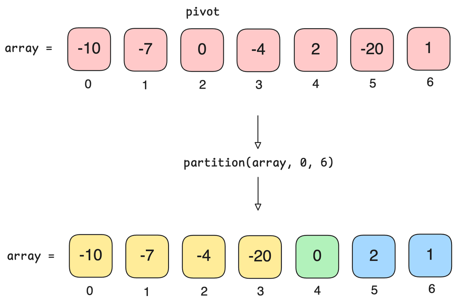
The key idea behind the recursive case is called partitioning. We pick any number, called pivot, then reorganize the array such that smaller numbers are placed on the left side, and bigger numbers are placed on the right side of pivot. Note that we don’t care about exact ordering of the numbers.
We will see how to implement the partition function later.
After partitioning the array, the pivot is placed at the position it would have in a sorted array, i.e. final_pivot_index. All that’s left is to sort the left section and the right section, and we can do that by calling the quicksort function recursively for each of them:
The left section is in range
[0, 3], so we do it by callingquicksort(array, 0, 3). Note thatfinal_pivot_index - 1 = 3.The right section is in range
[5, 6], so we do it by callingquicksort(array, 5, 6). Note thatfinal_pivot_index + 1 = 5.
By repeating this process, we will sort the entire array.
Partition function
Now let’s have a look at how the partition function works. We want to do this in-place since that’s one of the key benefits of quick sort. Let’s consider the following array of 8 elements:
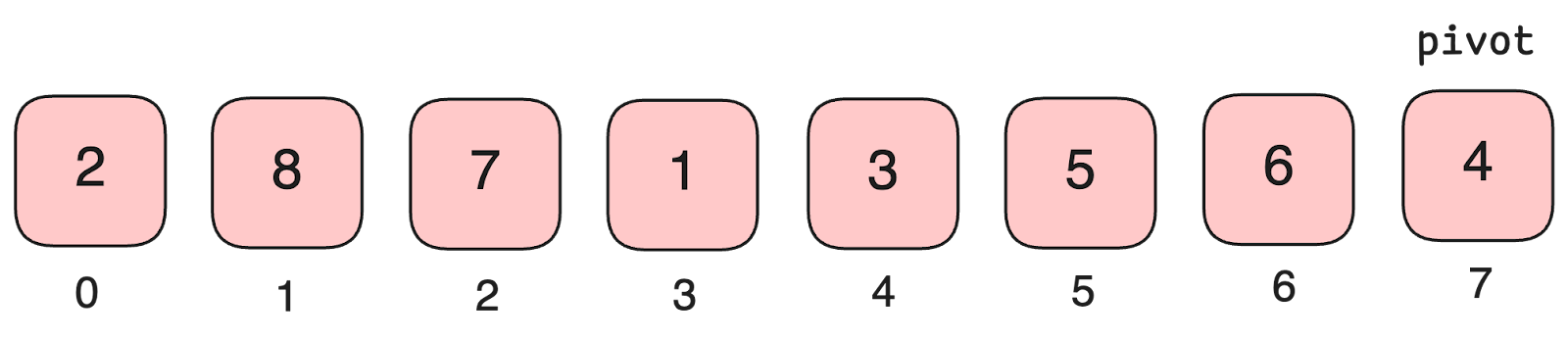
Let’s pick the last element as pivot. We will soon see how to pick any other element. In this case, the pivot is at index 7, which is number 4. We want all numbers that are less than 4 to be on the left, and all numbers that are greater than 4 to be on the right side.
How to do that?
We want to iterate over each element in the array and place it in either the left or the right group. This would have been easy if we were allowed to use additional memory, but since we want to do it in place, we also need to be smart about maintaining these groups.
To achieve this, we will maintain two pointers, such that elements at [0, i] are in the smaller group, while elements at [i + 1, j] are in the bigger group. The remaining elements are unscanned. Note that the next unscanned element is always at j+1 (see diagram 5).
Left pointer
i: It’s initialized such that the smaller group is empty.Right pointer
j: Scans through the array and maintains an invariant that all elements at[i+j, j]are in the bigger group.

If the next element is greater than the pivot, then we can simply increment j since the invariant still holds (see diagram 6). But what if the element is smaller than the pivot? How can we place it in the smaller group efficiently? Turns out this is trivial because we can extend both groups by 1 element, and swap the last two elements (see diagram 7).


We will repeat this until we reach the pivot element, then we swap the pivot with the first element from the bigger group. After this final step, we get the following:
All elements to the left of the pivot are smaller than the pivot.
All elements to the right of the pivot are larger.
The pivot is now in its final sorted position.

Duplicates
It’s straightforward to handle duplicates by putting them in one of the groups, usually the smaller group. However, there are optimization techniques that can improve performance for arrays with lots of duplicates, and we will look into these later.
Implementation
Partition Function
Let’s see how we could implement a partition function. Partition function returns the index of the pivot element because it’s required to recurse on the left and right groups.
function partition(array, left, right):
    pivot = array[right]
    i = left - 1

    for j = left to right - 1:
        if array[j] <= pivot:
            i = i + 1
            swap(array[i], array[j])

    swap(array[i + 1], array[right])
    return i + 1
Recursive Function
All that’s left is to implement a recursive function, and this is now trivial.
function quicksort(array, left, right):
    // Base case: only sort if the segment has more than 1 element
    if left < right:
        pivotIndex = partition(array, left, right)
        quicksort(array, left, pivotIndex - 1)
        quicksort(array, pivotIndex + 1, right)
We can also provide a polymorphic wrapper (for languages that support it) to not have to specify the range explicitly.
function quicksort(array):
    quicksort(array, 0, array.length - 1)
Time Complexity
Let’s consider the best case, worst case, and average case.
Worst Case
The worst case performance is O(N^2). For example, imagine an array that is already sorted. If we pick the last element as pivot the partition function would take O(N) and the array would remain unchanged. We would then call quicksort recursively for the first N-1 elements, and so on, leading to quadratic time complexity. If you want to be precise, it would take N*(N+1)/2 iterations.
Best Case
What about the best case scenario?
The best case scenario would be choosing the best pivot every time, which is median or a number closest to the median because both groups would have the same or closest number of elements after partitioning. As a result, subsequent recursive calls will have to sort half of the elements each.

What’s interesting is that at each level there are N iterations, and there are log N levels since we are always dividing by 2, meaning the time complexity is O(N lg N).
Average Case
It’s a bit tricky to think about this, but the average case is close to the best case performance but with potentially worse constant. When quicksort runs on a random input array, the partitioning is highly unlikely to happen in the same way at every level. We expect that some of the splits are reasonably well balanced, while some are fairly unbalanced.
I will leave the proof for another time.
Pivot Choice
Random Choice
Instead of choosing the last element every time, we can instead pick a pivot at random, then swap it with the last element for the above algorithm to work. Another way to implement this is to shuffle an array at random before attempting to sort it.
Median of Three
Another method for choosing a pivot is called the “median of three”. The idea is to choose 3 elements at random, then pick the median of those three. This way, we are reducing the probability of picking a bad pivot.
Dealing with duplicates: 3-way quicksort
Quicksort doesn’t perform well when there are a lot of duplicates, similar to an array that’s already sorted. There is an optimized version of the standard quicksort algorithm that is designed to handle arrays with many duplicate elements more efficiently, called 3-way quicksort.
In 3-way quicksort, we divide an array into three partitions, rather than two:
Elements less than pivot.
Elements equal to pivot.
Elements greater than pivot.
This significantly improves performance of quicksort for arrays that contain lots of duplicates. The implementation is based on the Dutch national flag problem that we will look at another time, i.e. it sorts an array of 0s, 1s, and 2s.
Memory Complexity
We said that quicksort can sort an array in-place. However, we may naively conclude that it doesn’t use any extra memory. However, that would be wrong because quicksort is a recursive algorithm and depending on how many levels of recursion are necessary, it may end up using up to the O(N) memory in the worst case.
Final Words
Thank you for getting all the way here. Hopefully this was intuitive and easy to understand. Don’t forget to share this with your friends, and I’ll see you in the next one.